Optimizing Traffic-Signal Timing on Big Bend Boulevard:
Data, Simulation and Validation
Summary. 4 County signals on Big Bend Blvd · weekday 5–6 PM · real County timing + counts · SUMO simulation validated (6/6 GEH < 5) · County plan 251 veh-h/h → model plan 179 (29% less) → simulator-optimized 170 (32% less). Preliminary: optimizer is our stand-in for the group's code.
1. Corridor and scope
4 signals, north → south · main road Big Bend (NB/SB), cross streets (EB/WB) · design hour weekday 5–6 PM · 13,738 veh/h total approach volume (summed over the 4 intersections).
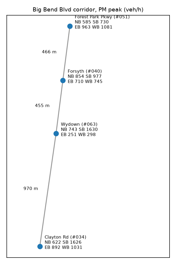
| link | length (m) | speed (m/s) | travel time \(\tau_i\) (s) |
|---|---|---|---|
| 051 → 040 | 466 | 13.4 | 34.8 |
| 040 → 063 | 455 | 15.7 | 29.1 |
| 063 → 034 | 970 | 15.7 | 62.0 |
Table 1. Links between consecutive signals (length from County coordinates; posted speeds from MoDOT 2025).
2. Data
2.1 Sources
| source | what we use | status |
|---|---|---|
| St. Louis County timing sheets (4 signals) | PM pattern 37: cycle, splits, offsets, yellow/all-red, phase sequence | measured |
| St. Louis County turning counts (4 signals) | 5–6 PM volumes by approach + L/T/R · Forsyth 2017, FPP 2021, Wydown 2025, Clayton 2026 | measured · verified vs sheet totals |
| MoDOT 2025 | lanes, speed limits | measured |
| County signal inventory | signal IDs, ownership, coordinates | measured |
| OpenStreetMap | approach lanes at the stop line | measured |
Every number is tagged measured / derived / assumed (appendix).
2.2 PM peak-hour volumes
| intersection | approach | veh/h | L | T | R | lanes | source |
|---|---|---|---|---|---|---|---|
| Forest Park Pkwy (#051) | NB | 585 | 0.16 | 0.71 | 0.13 | 2 | 051-forest-park-pkwy-2021-06-30.csv |
| Forest Park Pkwy (#051) | SB | 730 | 0.16 | 0.69 | 0.14 | 2 | 051-forest-park-pkwy-2021-06-30.csv |
| Forest Park Pkwy (#051) | EB | 963 | 0.25 | 0.69 | 0.07 | 3 | 051-forest-park-pkwy-2021-06-30.csv |
| Forest Park Pkwy (#051) | WB | 1081 | 0.14 | 0.66 | 0.20 | 3 | 051-forest-park-pkwy-2021-06-30.csv |
| Forsyth (#040) | NB | 854 | 0.19 | 0.68 | 0.13 | 2 | 040-forsyth-2017-03-03.csv |
| Forsyth (#040) | SB | 977 | 0.10 | 0.86 | 0.03 | 2 | 040-forsyth-2017-03-03.csv |
| Forsyth (#040) | EB | 710 | 0.07 | 0.42 | 0.51 | 3 | 040-forsyth-2017-03-03.csv |
| Forsyth (#040) | WB | 745 | 0.45 | 0.27 | 0.29 | 3 | 040-forsyth-2017-03-03.csv |
| Wydown (#063) | NB | 743 | 0.04 | 0.81 | 0.15 | 2 | 063-wydown-2025-09-26.csv |
| Wydown (#063) | SB | 1630 | 0.04 | 0.93 | 0.03 | 2 | 063-wydown-2025-09-26.csv |
| Wydown (#063) | EB | 251 | 0.15 | 0.49 | 0.36 | 2 | 063-wydown-2025-09-26.csv |
| Wydown (#063) | WB | 298 | 0.27 | 0.53 | 0.20 | 2 | 063-wydown-2025-09-26.csv |
| Clayton Rd (#034) | NB | 622 | 0.20 | 0.67 | 0.12 | 2 | 034-clayton-rd-2026-06-24.csv |
| Clayton Rd (#034) | SB | 1626 | 0.21 | 0.77 | 0.02 | 2 | 034-clayton-rd-2026-06-24.csv |
| Clayton Rd (#034) | EB | 892 | 0.12 | 0.63 | 0.25 | 4 | 034-clayton-rd-2026-06-24.csv |
| Clayton Rd (#034) | WB | 1031 | 0.23 | 0.66 | 0.11 | 4 | 034-clayton-rd-2026-06-24.csv |
Table 2. Measured approach volumes and turning shares, 5:00–6:00 PM. Lanes are approach lanes at the stop line.
2.3 Current signal timing (County, PM pattern)
| intersection | sheet | pattern | cycle (s) | offset (s) | phase splits (s) | Big Bend block | cross block | lost time L (s) |
|---|---|---|---|---|---|---|---|---|
| Forest Park Pkwy (#051) | October 21, 2026 | 37 | 120 | 10 | 1:18 2:42 3:18 4:42 5:18 6:42 7:18 8:42 | 60 | 60 | 23.4 |
| Forsyth (#040) | December 10, 2024 | 37 | 120 | 44 | 1:15 2:41 3:34 4:30 5:19 6:37 | 56 | 64 | 21.4 |
| Wydown (#063) | December 10, 2024 | 37 | 120 | 68 | 1:19 2:47 3:20 4:34 5:15 6:51 7:20 8:34 | 66 | 54 | 25.2 |
| Clayton Rd (#034) | May 12, 2026 | 37 | 120 | 23 | 1:27 2:39 3:20 4:34 5:24 6:42 7:23 8:31 | 66 | 54 | 27.0 |
Table 3. County timing, weekday PM. Splits include yellow and all-red. Lost time is the total clearance along the phase sequence.
3. Method
3.1 Pipeline
| step | what | input | output |
|---|---|---|---|
| 1 | Parse + verify County data | County PDFs (timing sheets, turning counts) | count CSVs, timing JSON; every count checked against the sheet's printed totals |
| 2 | Build corridor dataset | config, raw + measured data | corridor.json: every number tagged measured / derived / assumed |
| 3 | Optimizer input | corridor.json | optimizer_input.json / .csv for the model |
| 4 | SUMO network | corridor.json | 4 signals at real spacing, real approach lanes + left bays, posted speeds |
| 5 | SUMO demand | corridor.json | entry flows, measured turn shares, mid-block balancing flows |
| 6 | Timing plans | corridor.json, County timing | baselines, County current plan, formula optimum |
| 7 | Simulate | plans | 10 seeded runs per plan: delay, stops, throughput |
| 8 | Validate | runs vs counts | GEH per approach |
| 9 | Tables + figures | everything above | report tables, figures, this page |
Table 4. One command (./run_all.sh) reruns all steps.
3.2 Timing model
Signals \(i=1,\dots,N\) (north to south), approaches \(a\in\{\mathrm{NB},\mathrm{SB},\mathrm{EB},\mathrm{WB}\}\). Decision variables: common cycle \(C\), Big Bend green \(g_i\), offsets \(\theta_i\) (\(\theta_1=0\)). Solver: multistart SLSQP.
$$\min_{C,\;g,\;\theta}\;\; D(C,g,\theta)=\sum_{i=1}^{N}\sum_{a} q_{ia}\,d_{ia}(C,g,\theta)$$Webster delay for random arrivals, with green ratio \(\lambda=g/C\) and degree of saturation \(x=q/(\lambda s)\):
$$d_W=\frac{C(1-\lambda)^2}{2(1-\lambda x)}+\frac{x^2}{2q(1-x)}$$Platoon delay on Big Bend (arrivals released by the upstream signal, \(\tau_i\) = travel time, \(p\) = platoon share):
$$\phi=(\theta_{\mathrm{up}}+\tau-\theta_i)\bmod C,\qquad d_P(\phi)=\frac{1}{g_{\mathrm{up}}}\int_{\phi}^{\phi+g_{\mathrm{up}}} w(t)\,dt$$ $$d_{\mathrm{main}}=(1-p)\,d_{W,1}+p\,d_P(\phi)+d_{W,2}$$\(w(t)\) = wait of a car arriving at time \(t\) in the downstream cycle; \(d_{W,1}, d_{W,2}\) = first and second Webster terms.
Constraints:
$$C_{\min}\le C\le C_{\max},\qquad g_i\ge g_{\min},\qquad C-L_i-g_i\ge g_{\min},\qquad q_{ia}\,C\le x_{\max}\,s_{ia}\,g_{ia}$$Inputs from the signal sequence: lost time \(L_i\) = total yellow + all-red along the County phase sequence (critical ring); effective saturation flow \(s_{ia}=q_{ia}/Y_b\), where \(Y_b\) is the critical flow ratio of the phase block \(b\) serving approach \(a\):
$$Y_b=\max_{r\in\{1,2\}}\sum_{k\in b\cap r}\frac{q_k}{s_k},\qquad C_{\min}=60,\;C_{\max}=150\ \mathrm{s},\;\; x_{\max}=0.9,\;\; p=0.8$$3.3 Simulation
| setting | value |
|---|---|
| software | SUMO 1.28 |
| network | 4 signals at real spacing · real approach lanes · left-turn bays · posted speeds |
| demand | measured volumes + turn shares · mid-block balancing flows (Table 5) |
| signals | County phase sequence (incl. left arrows), scaled to each plan · right turn on red |
| run | 15 min warm-up + 60 min measured · 10 seeds per plan |
| metric | delay = time lost on corridor links + time waiting to enter (veh-h per hour) |
| link | direction | propagated veh/h | counted veh/h | balancing veh/h |
|---|---|---|---|---|
| 051-040 | SB | 716 | 977 | +261 |
| 051-040 | NB | 845 | 585 | -260 |
| 040-063 | SB | 1538 | 1630 | +92 |
| 040-063 | NB | 698 | 854 | +156 |
| 063-034 | SB | 1681 | 1626 | -55 |
| 063-034 | NB | 638 | 743 | +105 |
Table 5. Mid-block balancing flows: counted volume into a signal minus the volume propagated from the previous signal.
4. Validation
Simulated vs counted hourly volume, \(\mathrm{GEH}=\sqrt{2(M-C)^2/(M+C)}\) with \(M\) simulated, \(C\) counted · pass if \(\mathrm{GEH}<5\) · interior approaches: 6/6 pass.
| intersection | approach | kind | counted veh/h | simulated veh/h | GEH |
|---|---|---|---|---|---|
| Forest Park Pkwy (#051) | NB | interior | 585 | 611 | 1.08 |
| Forest Park Pkwy (#051) | SB | entry | 730 | 730 | 0.00 |
| Forest Park Pkwy (#051) | EB | entry | 963 | 963 | 0.00 |
| Forest Park Pkwy (#051) | WB | entry | 1081 | 1081 | 0.00 |
| Forsyth (#040) | NB | interior | 854 | 872 | 0.62 |
| Forsyth (#040) | SB | interior | 977 | 991 | 0.45 |
| Forsyth (#040) | EB | entry | 710 | 710 | 0.00 |
| Forsyth (#040) | WB | entry | 745 | 745 | 0.00 |
| Wydown (#063) | NB | interior | 743 | 774 | 1.14 |
| Wydown (#063) | SB | interior | 1630 | 1508 | 3.09 |
| Wydown (#063) | EB | entry | 251 | 251 | 0.00 |
| Wydown (#063) | WB | entry | 298 | 298 | 0.00 |
| Clayton Rd (#034) | NB | entry | 622 | 622 | 0.00 |
| Clayton Rd (#034) | SB | interior | 1626 | 1509 | 2.96 |
| Clayton Rd (#034) | EB | entry | 892 | 892 | 0.00 |
| Clayton Rd (#034) | WB | entry | 1031 | 1031 | 0.00 |
Table 6. Simulated vs counted volumes under the County's current timing (mean of 10 seeds).
5. Results
| plan | cycle (s) | SUMO delay, veh-h/h (mean ± sd) | vs County | stops / veh | throughput veh/h | formula delay | source |
|---|---|---|---|---|---|---|---|
| study1-sumo-loop | 124.7 | 169.9 ± 5.6 | -32% | 1.69 | 7861 | 115.1 | Study 1: Nelder-Mead on SUMO delay (120 evaluations x 2 seeds), warm start = formula optimum |
| formula-optimum-standin | 124.8 | 178.9 ± 3.5 | -29% | 1.74 | 7854 | 114.2 | stand-in for Michael+Noah: formula model, multistart SLSQP (formula.py) |
| sumo-coordinated | 150.0 | 203.3 ± 3.7 | -19% | 1.62 | 7842 | 128.6 | baseline: SUMO tlsCoordinator.py offsets on the common Webster plan |
| webster-per-light | 150.0 | 225.7 ± 4.4 | -10% | 2.01 | 7825 | — | baseline: Webster (1958) cycle + splits per light, uncoordinated |
| webster-common | 150.0 | 230.2 ± 3.8 | -8% | 1.77 | 7858 | 145.8 | baseline: common Webster cycle, Webster splits, offsets 0 |
| county-current | 120.0 | 251.3 ± 3.0 | +0% | 2.26 | 7852 | 963.2 | MEASURED: St. Louis County timing sheets, pattern 37 (PM weekday) |
| equal-split | 150.0 | 310.4 ± 8.4 | +24% | 2.28 | 7769 | 1830.3 | baseline: equal green to main and side, common Webster cycle, offsets 0 |
Table 7. All plans, 10 seeds each. formula-optimum-standin = our stand-in for the group's optimizer.
6. Study 1: simulator-in-the-loop vs formula model
| test | result |
|---|---|
| Does the formula rank plans like SUMO? ({s1['prediction']['n_plans']} random plans) | weakly · Spearman ρ = {s1['prediction']['spearman']:.2f} |
| Formula optimizer | {fo:.0f} veh-h/h · {s1['formula_optimizer']['seconds']} s |
| Simulator-in-the-loop (Nelder–Mead, {s1['sumo_loop']['evaluations']} evals) | {sl:.0f} veh-h/h · ~{s1['sumo_loop']['seconds']//60} min |
7. Interfaces for the optimizer
In: optimizer_input.json (\(q_{ia}, s_{ia}\) per approach; \(\tau_i\) per link; parameters) · Out: plan file with \(C\), \(g_i\), \(\theta_i\):
{ "name": "...", "C": 124.7,
  "lights": { "051": {"g_main": 37.0, "offset_s": 0.0},
              "040": {"g_main": 49.8, "offset_s": 52.7}, ... } }
\(g_i\) = g_main (Big Bend green, s) · cross-street green \(=C-L_i-g_i\) · \(\theta_i\) = offset_s (start of the Big Bend block relative to signal 1, s)
8. Modelling choices for the group to confirm
- Lost time \(L_i\) and saturation flow \(s_{ia}\) computed along the real signal sequence (\(L_i \approx 21\text{–}27\) s) · needs Michael + Noah's OK · switchable back.
- Real signals use left-turn arrows · simulation includes them · revisit "future work".
- Simulated network generated from measured geometry (full OpenStreetMap version jammed).
- Assumed: \(s_0 = 1800\) veh/h/lane · \(p = 0.8\) · 90 m left bays · right turn on red.
9. Status
| item | status |
|---|---|
| Real corridor data: County timing + turning counts for all 4 signals, verified | Done |
| SUMO simulation of the corridor, validated against counts | Done |
| All timing plans simulated (10 seeds each); results tables + figures | Done |
| Study 1 (simulator-in-the-loop vs formula model) | Done (first full run) |
| Reproducible code package + README (one command) | Done (data/simulation part) |
| Michael + Noah's optimizer (signal_opt.py) plugged in | Open: stand-in used |
| Group agreement on the modelling choices in §8 | Open |
| Written report sections (Data, Setup, Study 1) | Open |
| Full report (8–12 pp), Contributions, submission + code to TA | Open |
10. Reproducing the results
cd pipeline
./run_all.sh                                   # data, network, plans, 10-seed runs, validation, tables
.venv/bin/python src/study1.py --n-random 30 --budget 120   # Study 1
Inputs: data/, config/ · outputs: build/ (regenerated).
Appendix: where every number comes from
| where | input | value | source | evidence |
|---|---|---|---|---|
| #051 NB | volume | 585 veh/h | measured | St. Louis County turning-movement count 051-forest-park-pkwy-2021-06-30.csv, 17:00-18:00 (L 95, T 415, R 75) |
| #051 NB | saturation flow (model) | 2632 veh/h | derived | effective: q / Y_block, Y_block = 0.222 = critical flow ratio of this block along the County phase sequence (measured volumes, lanes; 1800 veh/h/lane) |
| #051 SB | volume | 730 veh/h | measured | St. Louis County turning-movement count 051-forest-park-pkwy-2021-06-30.csv, 17:00-18:00 (L 120, T 505, R 105) |
| #051 SB | saturation flow (model) | 3285 veh/h | derived | effective: q / Y_block, Y_block = 0.222 = critical flow ratio of this block along the County phase sequence (measured volumes, lanes; 1800 veh/h/lane) |
| #051 EB | volume | 963 veh/h | measured | St. Louis County turning-movement count 051-forest-park-pkwy-2021-06-30.csv, 17:00-18:00 (L 239, T 661, R 63) |
| #051 EB | saturation flow (model) | 2457 veh/h | derived | effective: q / Y_block, Y_block = 0.392 = critical flow ratio of this block along the County phase sequence (measured volumes, lanes; 1800 veh/h/lane) |
| #051 WB | volume | 1081 veh/h | measured | St. Louis County turning-movement count 051-forest-park-pkwy-2021-06-30.csv, 17:00-18:00 (L 148, T 713, R 220) |
| #051 WB | saturation flow (model) | 2758 veh/h | derived | effective: q / Y_block, Y_block = 0.392 = critical flow ratio of this block along the County phase sequence (measured volumes, lanes; 1800 veh/h/lane) |
| #051 | lost time L | 23.4 s | measured | County sheet, signal_sequence |
| #040 NB | volume | 854 veh/h | measured | St. Louis County turning-movement count 040-forsyth-2017-03-03.csv, 17:00-18:00 (L 164, T 580, R 110) |
| #040 NB | saturation flow (model) | 2556 veh/h | derived | effective: q / Y_block, Y_block = 0.334 = critical flow ratio of this block along the County phase sequence (measured volumes, lanes; 1800 veh/h/lane) |
| #040 SB | volume | 977 veh/h | measured | St. Louis County turning-movement count 040-forsyth-2017-03-03.csv, 17:00-18:00 (L 102, T 842, R 33) |
| #040 SB | saturation flow (model) | 2924 veh/h | derived | effective: q / Y_block, Y_block = 0.334 = critical flow ratio of this block along the County phase sequence (measured volumes, lanes; 1800 veh/h/lane) |
| #040 EB | volume | 710 veh/h | measured | St. Louis County turning-movement count 040-forsyth-2017-03-03.csv, 17:00-18:00 (L 51, T 296, R 363) |
| #040 EB | saturation flow (model) | 2635 veh/h | derived | effective: q / Y_block, Y_block = 0.269 = critical flow ratio of this block along the County phase sequence (measured volumes, lanes; 1800 veh/h/lane) |
| #040 WB | volume | 745 veh/h | measured | St. Louis County turning-movement count 040-forsyth-2017-03-03.csv, 17:00-18:00 (L 333, T 198, R 214) |
| #040 WB | saturation flow (model) | 2765 veh/h | derived | effective: q / Y_block, Y_block = 0.269 = critical flow ratio of this block along the County phase sequence (measured volumes, lanes; 1800 veh/h/lane) |
| #040 | lost time L | 21.4 s | measured | County sheet, signal_sequence |
| #063 NB | volume | 743 veh/h | measured | St. Louis County turning-movement count 063-wydown-2025-09-26.csv, 17:00-18:00 (L 33, T 602, R 108) |
| #063 NB | saturation flow (model) | 1639 veh/h | derived | effective: q / Y_block, Y_block = 0.453 = critical flow ratio of this block along the County phase sequence (measured volumes, lanes; 1800 veh/h/lane) |
| #063 SB | volume | 1630 veh/h | measured | St. Louis County turning-movement count 063-wydown-2025-09-26.csv, 17:00-18:00 (L 64, T 1511, R 55) |
| #063 SB | saturation flow (model) | 3596 veh/h | derived | effective: q / Y_block, Y_block = 0.453 = critical flow ratio of this block along the County phase sequence (measured volumes, lanes; 1800 veh/h/lane) |
| #063 EB | volume | 251 veh/h | measured | St. Louis County turning-movement count 063-wydown-2025-09-26.csv, 17:00-18:00 (L 37, T 124, R 90) |
| #063 EB | saturation flow (model) | 1537 veh/h | derived | effective: q / Y_block, Y_block = 0.163 = critical flow ratio of this block along the County phase sequence (measured volumes, lanes; 1800 veh/h/lane) |
| #063 WB | volume | 298 veh/h | measured | St. Louis County turning-movement count 063-wydown-2025-09-26.csv, 17:00-18:00 (L 80, T 159, R 59) |
| #063 WB | saturation flow (model) | 1824 veh/h | derived | effective: q / Y_block, Y_block = 0.163 = critical flow ratio of this block along the County phase sequence (measured volumes, lanes; 1800 veh/h/lane) |
| #063 | lost time L | 25.2 s | measured | County sheet, signal_sequence |
| #034 NB | volume | 622 veh/h | measured | St. Louis County turning-movement count 034-clayton-rd-2026-06-24.csv, 17:00-18:00 (L 126, T 419, R 77) |
| #034 NB | saturation flow (model) | 1460 veh/h | derived | effective: q / Y_block, Y_block = 0.426 = critical flow ratio of this block along the County phase sequence (measured volumes, lanes; 1800 veh/h/lane) |
| #034 SB | volume | 1626 veh/h | measured | St. Louis County turning-movement count 034-clayton-rd-2026-06-24.csv, 17:00-18:00 (L 344, T 1244, R 38) |
| #034 SB | saturation flow (model) | 3816 veh/h | derived | effective: q / Y_block, Y_block = 0.426 = critical flow ratio of this block along the County phase sequence (measured volumes, lanes; 1800 veh/h/lane) |
| #034 EB | volume | 892 veh/h | measured | St. Louis County turning-movement count 034-clayton-rd-2026-06-24.csv, 17:00-18:00 (L 110, T 558, R 224) |
| #034 EB | saturation flow (model) | 3226 veh/h | derived | effective: q / Y_block, Y_block = 0.276 = critical flow ratio of this block along the County phase sequence (measured volumes, lanes; 1800 veh/h/lane) |
| #034 WB | volume | 1031 veh/h | measured | St. Louis County turning-movement count 034-clayton-rd-2026-06-24.csv, 17:00-18:00 (L 237, T 685, R 109) |
| #034 WB | saturation flow (model) | 3729 veh/h | derived | effective: q / Y_block, Y_block = 0.276 = critical flow ratio of this block along the County phase sequence (measured volumes, lanes; 1800 veh/h/lane) |
| #034 | lost time L | 27.0 s | measured | County sheet, signal_sequence |
| model | p | 0.8 | assumed | model defaults from the Nov 10 formulation |
| model | g_min_s | 10.0 | assumed | model defaults from the Nov 10 formulation |
| model | C_min_s | 60.0 | assumed | model defaults from the Nov 10 formulation |
| model | C_max_s | 150.0 | assumed | model defaults from the Nov 10 formulation |
| model | x_max | 0.9 | assumed | model defaults from the Nov 10 formulation |
| network | left-turn bay length | 90 m | assumed | typical urban 75–100 m; not measured |